Rossby Wave Sources Diagnostic Package
Last update 04/15/2021
ENSO Rossby wave sources (ENSO_RWS) diagnostic package consists of four levels. With a focus on identifying leading processes that determine ENSO-induced global teleconnection, particularly the Pacific North American (PNA) pattern, the main module of the POD estimates basic state flow properties at an appropriate tropospheric upper-level and solves the barotropic vorticity equation to estimate various terms that contribute to the total anomalous RWS. In that pursuit, the ENSO-RWS POD is applied to monthly data (climate model or reanalysis products), and RWS terms are estimated for “composite” El Niño or La Nina events. To attain robust “composite” results a reasonable sample of ENSO winters is needed. However, the POD can be applied even for a single El Niño winter (e.g., when applied to seasonal prediction models). Similarly, the POD is applicable to any number of pressure levels (e.g., to identify the level at which maximum upper-level divergence and associated RWS are located). Here, reanalysis products (e.g., ERA-Interim) are considered as observations and diagnostics obtained from ERA-Interim and other reanalysis products are used for model validation. In this general document, brief descriptions of the four levels of the POD are provided, and detailed information is provided at each level. For the four levels of diagnostics, selected results are illustrated here.
The POD works efficiently if the model data contain a sufficient number of El Niño or La Nina events. Predigested results are available for both El Niño and La Nina composites.
Version and contact information
Version 1, 03/09/2021
PI: Dr. H. Annamalai (IPRC/SOEST University of/ Hawaii; hanna@hawaii.edu )
Current developer: Jan Hafner (IPRC/SOEST University of Hawaii; jhafner@hawaii.edu)
Open source copyright agreement
The MDTF framework is distributed under the LGPLv3 license (see LICENSE.txt).
Functionality
The current package consists of the following functionalities:
Basic ENSO diagnostics performed by script LEVEL_01.py
Climatological flow properties script LEVEL_02.py
Rossby wave source terms performed by script LEVEL_03.py
Scatter plots as metrics to assess models performed by script LEVEL_04.py
As a module of the MDTF code package, all scripts to perform the four levels can be found here: ~/diagnostics/ENSO_RWS/
The pre-digested observational data for model validation can be found here: ~/diagnostics/inputdata/obs_data/ENSO_RWS/
Required programming language and libraries
This package is coded in Python 3.8.5 and requires the following packages: numpy, os, math, xarray, netcdf4.
The pre-processing and plotting are coded in NCAR Command Language Version 6.5.0.
Required model output variables and their corresponding units
The following model fields are required as monthly data:
4-D variables (longitude, latitude, pressure level, time):
zg: HGT geopotential height (m)
ua: U wind component [m/s]
va: V wind component [m/s]
ta: Temperature (K)
wap: Vertical velocity (Pa/s)
3-D variables (longitude, latitude, time):
pr: Precipitation (k/m2/s)
ts: Surface temperature (K)
More details can be found in the README_general.pdf document.
References
1. Annamalai, H., R. Neale and J. Hafner: ENSO-induced teleconnection: development of PODs to assess Rossby wave sources in climate models (in preparation).
2. R. Neale and H. Annamalai: Rossby wave sources and ENSO- induced teleconnections in CAM6 model development versions and associated vertical processes (in preparation).
More about ENSO_RWS
Rossby Wave Source POD to assess ENSO-induced teleconnection (ENSO_RWS)
The NOAA-MDTF Rossby Wave Source (RWS) Process Oriented Diagnostic (POD) package fills a critical gap in the diagnostics tools available to climate model developers. In both basic-state and anomalous conditions, changes in the response of moist processes in model either parameterization modifications or tuning and calibration can often change the nature of the seasonal distributions of tropical precipitation and associated heating, and by association moistening and divergence profiles. While validation of precipitation is straightforward, an understanding of the circulation consequences in the tropics and the extra-tropics is not.
The RWS POD developed here will help to address this critical validation gap by quantifying the roles of changing ambient flow properties (basic state climatological features), and anomalous upper tropospheric divergent patterns in the generation and radiation of planetary stationary Rossby waves. This will be particularly important in coupled configuration development, since changes to the atmosphere model configuration can lead to complex coupled feedback modifying not only the mean climate, but the response during ENSO events.
A further role this POD plays is in determining the potential for generated interactions to influence the United States, and whether a particular model version has prediction utility.
Few take home messages to model development include:
Ambient flow properties (e.g., restoring force for stationary Rossby waves)
Perturbations to local Hadley and planetary east-west Walker circulations (generation of Rossby wave sources)
Location and intensity of anomalous Rossby wave sources and their dependence on both ambient and anomalous circulation conditions (principal Rossby wave sources)
Radiation of Rossby waves in the presence of ambient flow properties (great circle path)
To infer ENSO-induced seasonal anomalies over North America (prediction utility)
Level 1 – Basic ENSO diagnostics
Identify ENSO winters and construct seasonal composite anomalies for relevant variables (e.g., anomalous precipitation, circulation, geopotential height to estimate standardized PNA index).
Reference index (e.g., Nino3.4 SST)
Seasonal averages
Based on a reference ENSO index (e.g., area-averaged SST anomalies over the Nino3.4 region), seasonal composites of variables relevant to ENSO-induced global teleconnection at an appropriate tropospheric upper-level are constructed. Fig. 1 shows composite anomalous precipitation (shaded), 200hPa divergence/convergence (contour/hatching) and 200hPa divergent wind (vector) for boreal winter (DJF) season during El Niño constructed from GFDL-CAM4 AMIP simulations performed for the period 1980-2014 (Fig. 1a) and ERA-interim (Fig. 1b).
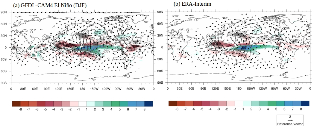
Figure 1: El Niño winter (DJF) composites of precipitation anomalies (shaded; mm/day), anomalous 200hPa convergence/divergence (contours/hatching in units of 10-6 s-1) and anomalous 200hPa divergent wind anomalies (m/s) constructed from: (a) AMIP simulation of GFDL-AM4 performed for the period 1980-2014 and (b) ERA-interim. Reference wind vector is also shown.
More details on Level 1 diagnostics can be found in the README_LEVEL_01.pdf document located in ~/diagnostics/ENSO_RWS/doc.
Level 2 – Climatological flow and wave properties (basic-state/ambient flow) diagnostics
Regarding to basic or climatological flow properties, restoring effect for Rossby waves (β*) that is dependent on meridional gradient in absolute vorticity (β) and meridional curvature of the zonal flow or gradients in relative vorticity \(\frac{\partial^{2}{{U}}}{\partial{y}^{2}}\) and resultant stationary wave number (\(K_{s}\)) are diagnosed. These ambient flow properties determine generation and propagation of stationary Rossby waves.
Mathematical expressions for β* and \(K_{s}\) are given by:
\(\beta_{*} = \beta - \frac{\partial^{2}{{U}}}{\partial{y}^{2}}\) (1)
\(K_{s} = \ \Big( { \beta_{*}} / {U} \Big)\)1/2 (2)
where β is latitudinal variations in planetary vorticity (\(f\)), \(\acute{U}\) is the basic-state zonal wind velocity, and \(\frac{\partial^{2}{{U}}}{\partial{y}^{2}}\) is the curvature of the ambient zonal flow. Stationary Rossby waves are possible if the flow is westerly (\(\acute{U}\) positive) and \(\beta_{*}\) is positive.
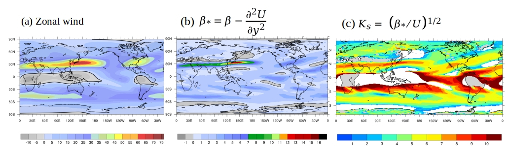
Figure 2: GFDL-AM4 simulated ambient flow properties at 200hPa for boreal winter (December – February): (a) zonal wind (m/s); (b) \(\beta_{}\)(10-11m-1s-1) and (c) stationary wavenumber. In (a and b), negative values are shaded gray and zero contour is shown as thick line. In (c) unspecified or singular values of wavenumber is shown as white.
More details on Level 2 diagnostics can be found in the README_LEVEL_02.pdf document located in ~/diagnostics/ENSO_RWS/doc.
Level 3 – Rossby wave sources (for composite ENSO)
Explicitly solves barotropic vorticity budget and the leading terms contributing to the total anomalous Rossby wave sources (\(\text{RW}S^{'}\)) are quantified. The mathematical expression for \(\text{RW}S^{'}\) is given by:

Here, \(\xi\) and \(v_{\chi}\) correspond to absolute vorticity and divergent component of the wind, respectively. The overbar represents seasonal mean and the prime refers to seasonal anomalies. The first term in \(\text{RW}S^{'}\)corresponds to stretching due to anomalous divergence, and the second term accounts for advection of climatological gradient in \(\xi\) by the anomalous divergent wind. The third and fourth terms account for transient eddy convergence of vorticity, and their contributions to \(\text{RW}S^{'}\) is small but non-negligible.
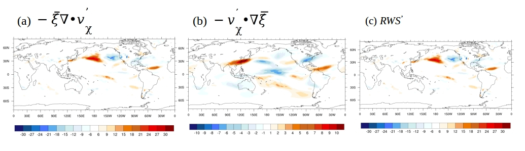
Figure 3: Anomalous Rossby wave sources (10-11s-2) due to: (a) stretching term; (b) anomalous divergent wind advecting gradient in climatological absolute vorticity and (c) all the four terms (equation 3). Results shown are for composite El Niño winters (DJF) simulated by GFDL-AM4 AMIP simulations.
More details on Level 3 diagnostics can be found in the README_LEVEL_03.pdf document located in ~/diagnostics/ENSO_RWS/doc.
Level 4 – Scatter plots for assessing models’ performance (Metrics).
Note that if diagnostics from multiple models are sought to assess systematic errors across all models and/or compare and contrast a selected model’s performance with other models then the results can be displayed as scatter plots between variables that are physically linked. At this level, results from Levels 1-3 are condensed into scatter plots. Specifically, estimates of leading anomalous RWS terms are plotted against equatorial precipitation and/or standardized PNA index (defined from 200hPa height anomalies).
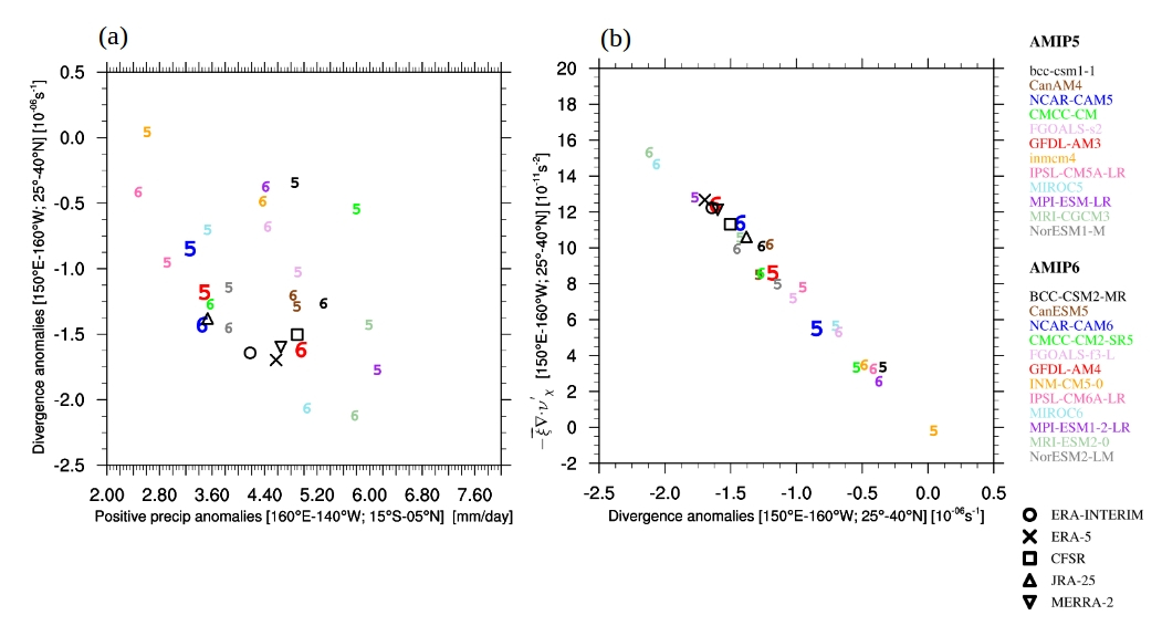
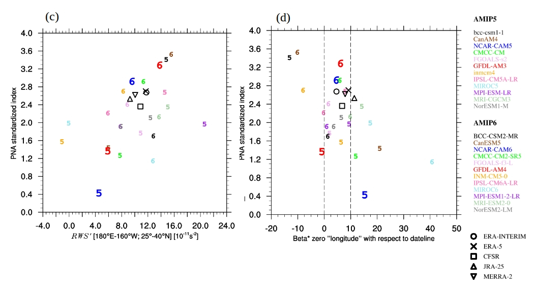
Figure 4: Scatter plots between (a) anomalous equatorial Pacific precipitation (160oE-140oW; 15oS-0) and 200hPa divergence (150oE-160oW; 25oN-40oN); (b) anomalous 200hPa divergence and \(\text{RW}S\)due to stretching term (150oE-160oW; 25oN-40oN); (c) anomalous total \(\text{RW}S^{'}\) east of the dateline (180oE-160oW; 25o-40oN) and standardized PNA index and (d) 200hPa climatological \(\beta_{}\)zero value longitude with respect to dateline and standardized PNA index. Results shown are for composite El Niño winters (DJF) simulated by AMIP5/6 models. In the panels, number 5 corresponds to AMIP5 and 6 corresponds to AMIP6 models, and the color of the numbers correspond to the model’s name.
More details on Level 4 diagnostics can be found in the README_LEVEL_04.pdf document located in ~/diagnostics/ENSO_RWS/doc.