Rich Neale’s Blocking Diagnostic Documentation
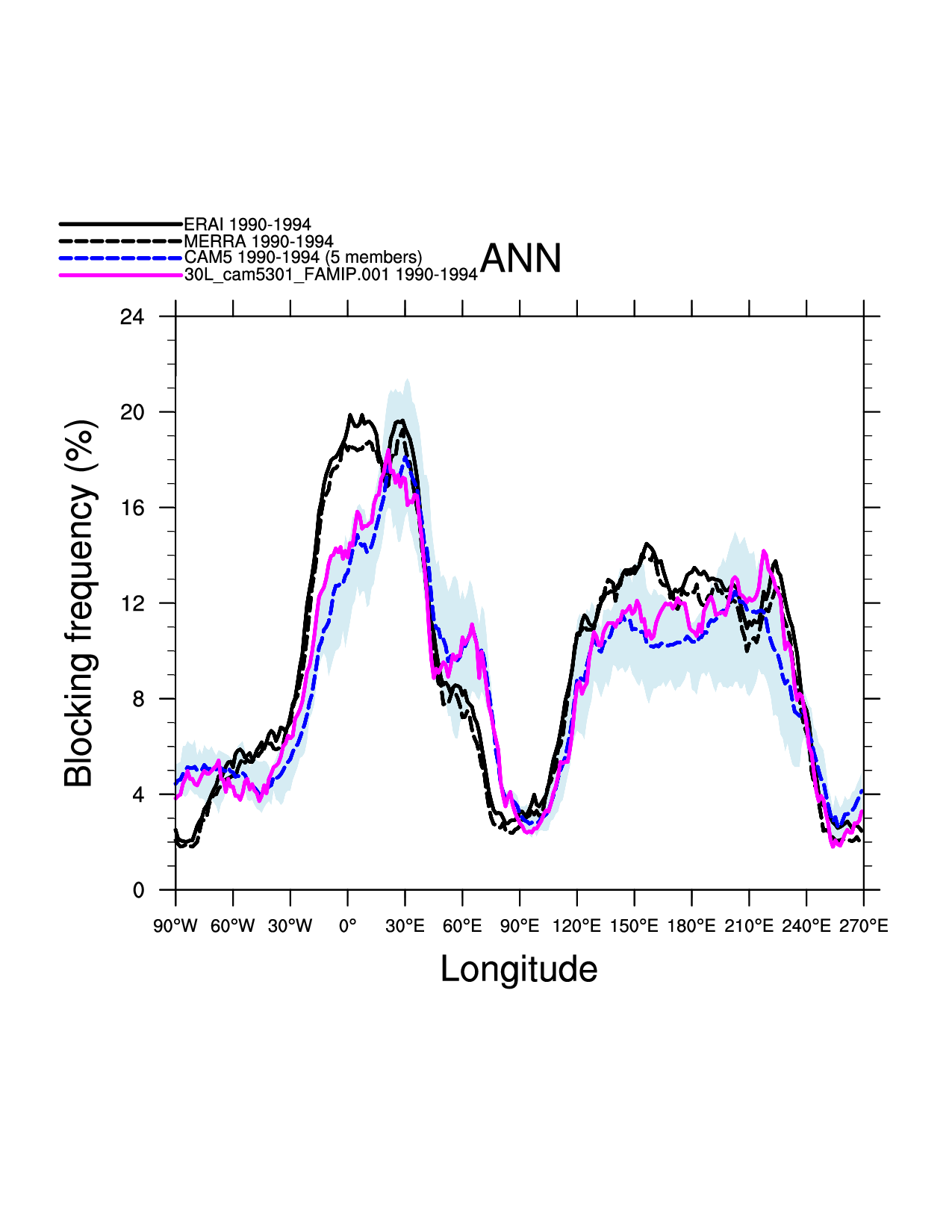
Evaluate blocking frequency by season as determined by the meridional gradient above a threshold value of daily 500mb height following D’Andrea et al (1998) and a 2D variant of the above where lat and lon daily 500-mb thresholds are considered Davini et al
Version & Contact info
Open source copyright agreement
The MDTF framework is distributed under the LGPLv3 license (see LICENSE.txt)
Functionality
Required programming language and libraries
Python 3
NCL (usual NCAR/CESM packages: contributed, gsn_code, gsn_csm)
Required model output variables
Geopotential height at 500 milibars or 3D field with air pressure available
Settings/Environment Variables
There are two sets of environment variables that can be set in the input jsonc file:
What to compare input case(s) against:
observational products from ERAI & MERRA. Can be turned on or off together. Default: On Years used can be controlled individually
three CESM 5-member ensembles (CAM3, CAM4, CAM5) which can be turned on or off individually. Default: CAM5 only. (Note that the code runs with these but the html file does not yet respond to this. Therefore the POD will fail to link the figures if non-default options are used)
Variable name
Default
“MDTF_BLOCKING_OBS” : “True”, //both ERA & MERRA (not possible to choose individually yet) “MDTF_BLOCKING_OBS_USE_CASE_YEARS”: “False”, //if False, must set ERA/MERRA/CAM5 FIRST/LAST-YRS below “MDTF_BLOCKING_OBS_ERA_FIRSTYR” : 2010, “MDTF_BLOCKING_OBS_ERA_LASTYR” : 2014, “MDTF_BLOCKING_OBS_MERRA_FIRSTYR” : 2009, “MDTF_BLOCKING_OBS_MERRA_LASTYR” : 2011, “MDTF_BLOCKING_OBS_CAM5_FIRSTYR” : 1979, “MDTF_BLOCKING_OBS_CAM5_LASTYR” : 2007, “MDTF_BLOCKING_CAM3” : “False”, //if True, will run but doesn’t show on webpage “MDTF_BLOCKING_CAM4” : “False”, //if True, will run but doesn’t show on webpage “MDTF_BLOCKING_CAM5” : “True”, “MDTF_BLOCKING_READ_DIGESTED” : “True”, // if True, files must be available “MDTF_BLOCKING_WRITE_DIGESTED” : “False”, // if True, writes out case data as digested. requires READ_DIGESTED = False “MDTF_BLOCKING_WRITE_DIGESTED_DIR”: “”, // default output directory for digested data “MDTF_BLOCKING_DEBUG” : “False” // reduces number of ensemble members to 2 for quicker execution
- REMOVED:
“MDTF_BLOCKING_COMPARE_LONG_YEARS” use instead the more detailed variables above
Variables to control reading or writing of digested data
MDTF_BLOCKING_READ_DIGESTED (Default True)If True, the POD looks for digested data for the obs & CAM ensembles Digested means the data has been processed by this POD into the block_time variable name and format (seeMDTF_BLOCKING_WRITE_DIGESTEDbelow)(MDTF_BLOCKING_READ_DIGESTED = False)If False, the POD looks for raw data (Z500(time,lat,lon)).The POD is not currently capable of running with a mix of digested and undigested (other than the undigested MDTF input case). If the user desires this, it is recommended to run only the components that are not digested, and write out digested. Then re-running with MDTF_BLOCKING_READ_DIGESTED will work.
It is not yet possible to run the MDTF input case with digested data, although it is possible to write it out.
OBS/CAM file name & dir expectations:Digested: obs_data/blocking/ERAI/ERAI.z500.day. digested .ncUndigested: obs_data/blocking/undigested/ERAI/ERAI.z500.day.ncMDTF_BLOCKING_WRITE_DIGESTED (Default False)If True, whatever data was read in raw will be written out digested. This is how a user can make a new digested file, whether obs, a new case or ensemble, or a previous MDTF input case to compare against.
Code Overview
The POD is called by a python wrapper script, blocking_neale.py which
calls blocking.ncl.
blocking.ncl summary:
Read all case data from environmental variables and store it in
all_casesstructureall_cases = blocking_get_all_case_info()is a data structure defined in blocking_funcs.ncl which contains arrays of length number of cases (mdtf case + obs cases + comparison models) and contains the following components:case_names(short names; for ensembles these are the group name repeated length ncase)file_names(paths to files for each case (distinct for each ensemble member))var_names(what the variables are named in the datasets)years_run0, years_run1(start and stop years for each case)plot_colorshard-coded for consistency from run to run
Sets up figures that need to be done before each season is processed To be done
Loops over seasons (tested on ANN. DJF & JJA not tested)
Loops over files. File settings obtained by
file_opts = extract_file_opts(all_cases,ifile)If
MDTF_BLOCKING_READ_DIGESTED = TrueCalls
blocking_digested.ncl:open_digested()to openfile_opts@file_name(set inblocking_funcs.ncl:set_and_check_file_names()) readsblock_time = f_dig->$var_name$(idays,:)elsereads raw Z500 data usingvar_in_p = blocking_readfile_origand computes the blocking index asblock_time(lon)following Tibaldi and Molteni (1990)
If
MDTF_BLOCKING_WRITE_DIGESTEDOptionally writesblock_timeout as digested datacomputes
block_daysas sum of all days that were blocked over the entire time period, as a function of longitude (as well as std for ensembles)block_stdandblock_freqto be blocked/all days.for season
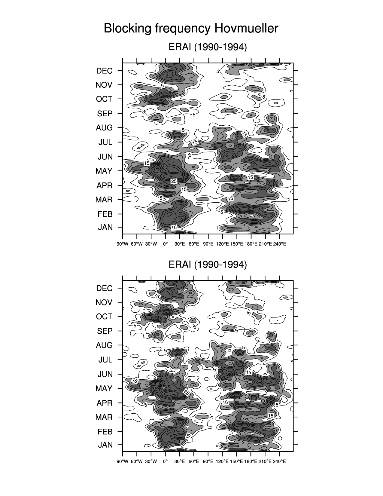
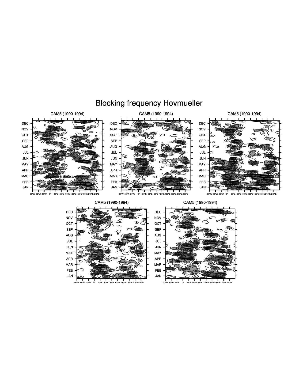
ANN(annual) only, calculate daily frequencyblock_freq_yr(ndoys,nlons)for Hovmüllers, smoothed by smth9_Wrap
Loops over ensemble groups for figures
Store data in arrays
block_freq_aves_p, block_freq_min_p/max_pSet more plotting resources
res_mIndividual (Hovmueller figures)
plot_t(ifile) = gsn_csm_hov(wks_ens_page, lonPivot(block_freq_yr,270.), res_t)Combined seasonal figure (one figure with a line for each dataset)
plot(ip) = gsn_csm_xy (wks,block_freq_aves_p&lon,block_freq_aves_p,res_m)
Figures
References
1. Tibaldi and Molteni (1990): On the operational predictability of blocking. Tellus A: Dynamic Meteorology and Oceanography, 42 (3), 343-365, doi:10.3402/tellusa.v42i3.11882.
2. D’Andrea, F., Tibaldi, S., Blackburn, M. et al. (1998): Northern Hemisphere atmospheric blocking as simulated by 15 atmospheric general circulation models in the period 1979–1988. Climate Dynamics, 14, 385–407 doi:10.1007/s003820050230.
3. Davini, P., Cagnazzo, C., Neale, R., and Tribbia, J. (2012): Coupling between Greenland blocking and the North Atlantic Oscillation pattern, Geophys. Res. Lett., 39, L14701, doi:10.1029/2012GL052315.